3.1.1. Image Augmentation

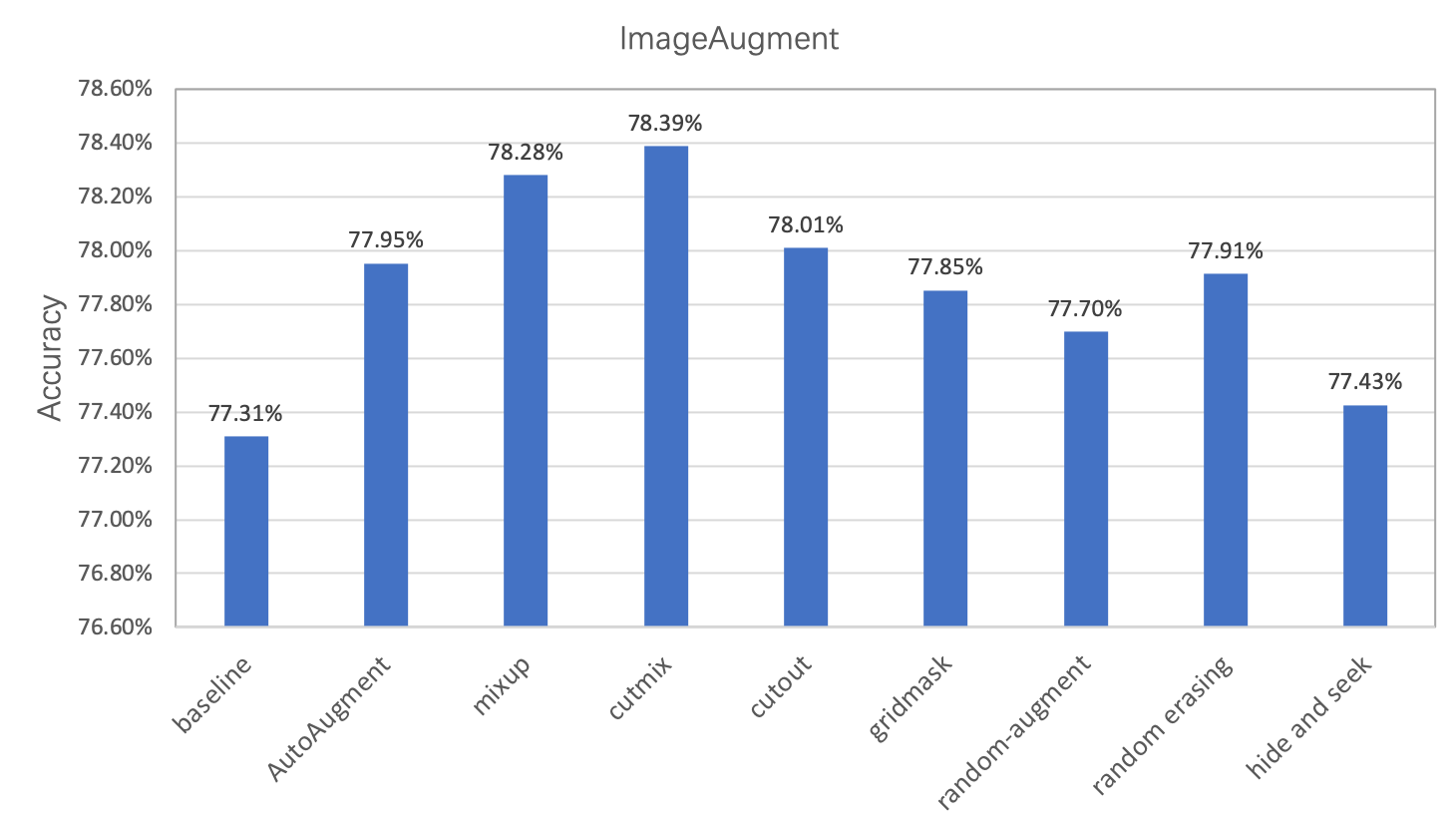
Image augmentation is a commonly used regularization method in image classification task, which is often used in scenarios with insufficient data or large model. In this chapter, we mainly introduce 8 image augmentation methods besides standard augmentation methods. Users can apply these methods in their own tasks for better model performance. Under the same conditions, These augmentation methods’ performance on ImageNet1k dataset is shown as follows.

3.1.2. Common image augmentation methods

If without special explanation, all the examples and experiments in this chapter are based on ImageNet1k dataset with the network input image size set as 224.

The standard data augmentation pipeline in ImageNet classification tasks contains the following steps.

1. Decode image, abbreviated as ImageDecode.
2. Randomly crop the image to size with 224x224, abbreviated as RandCrop.
3. Randomly flip the image horizontally, abbreviated as RandFlip.
4. Normalize the image pixel values, abbreviated as Normalize.
5. Transpose the image from [224, 224, 3](HWC) to [3, 224, 224](CHW), abbreviated as Transpose.
6. Group the image data([3, 224, 224]) into a batch([N, 3, 224, 224]), where N is the batch size. It is abbreviated as Batch.

Compared with the above standard image augmentation methods, the researchers have also proposed many improved image augmentation strategies. These strategies are to insert certain operations at different stages of the standard augmentation method, based on the different stages of operation. We divide it into the following three categories.

1. Transformation. Perform some transformations on the image after RandCrop, such as AutoAugment and RandAugment.
2. Cropping. Perform some transformations on the image after Transpose, such as CutOut, RandErasing, HideAndSeek and GridMask.
3. Aliasing. Perform some transformations on the image after Batch, such as Mixup and Cutmix.

The following table shows more detailed information of the transformations.

Method	Input	Output	Auto- Augment[1]	Rand- Augment[2]	CutOut[3]	Rand Erasing[4]	HideAnd- Seek[5]	GridMask[6]	Mixup[7]	Cutmix[8]
Image Decode	Binary	(224, 224, 3) uint8	Y	Y	Y	Y	Y	Y	Y	Y
RandCrop	(:, :, 3) uint8	(224, 224, 3) uint8	Y	Y	Y	Y	Y	Y	Y	Y
Process	(224, 224, 3) uint8	(224, 224, 3) uint8	Y	Y	-	-	-	-	-	-
RandFlip	(224, 224, 3) uint8	(224, 224, 3) float32	Y	Y	Y	Y	Y	Y	Y	Y
Normalize	(224, 224, 3) uint8	(3, 224, 224) float32	Y	Y	Y	Y	Y	Y	Y	Y
Transpose	(224, 224, 3) float32	(3, 224, 224) float32	Y	Y	Y	Y	Y	Y	Y	Y
Process	(3, 224, 224) float32	(3, 224, 224) float32	-	-	Y	Y	Y	Y	-	-
Batch	(3, 224, 224) float32	(N, 3, 224, 224) float32	Y	Y	Y	Y	Y	Y	Y	Y
Process	(N, 3, 224, 224) float32	(N, 3, 224, 224) float32	-	-	-	-	-	-	Y	Y

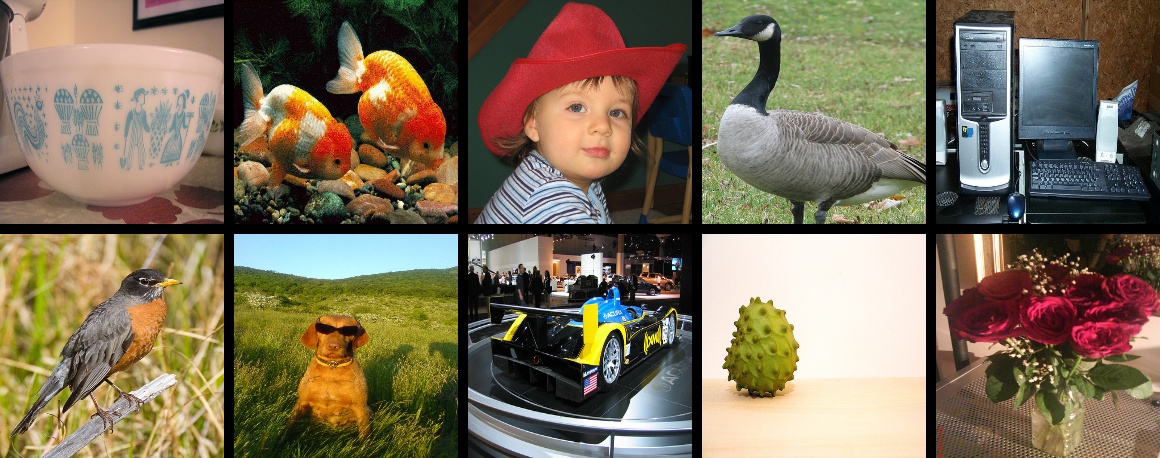
PaddleClas integrates all the above data augmentation strategies. More details including principles and usage of the strategies are introduced in the following chapters. For better visualization, we use the following figure to show the changes after the transformations. And RandCrop is replaced withResize for simplification.

3.1.3. Image Transformation

Transformation means performing some transformations on the image after RandCrop. It mainly contains AutoAugment and RandAugment.

3.1.3.1. AutoAugment

Address：https://arxiv.org/abs/1805.09501v1

Github repo：https://github.com/DeepVoltaire/AutoAugment

Unlike conventional artificially designed image augmentation methods, AutoAugment is an image augmentation solution suitable for a specific data set found by certain search algorithm in the search space of a series of image augmentation sub-strategies. For the ImageNet dataset, the final data augmentation solution contains 25 sub-strategy combinations. Each sub-strategy contains two transformations. For each image, a sub-strategy combination is randomly selected and then determined with a certain probability Perform each transformation in the sub-strategy.

In PaddleClas, AutoAugment is used as follows.

from ppcls.data.imaug import DecodeImage
from ppcls.data.imaug import ResizeImage
from ppcls.data.imaug import ImageNetPolicy
from ppcls.data.imaug import transform

size = 224

decode_op = DecodeImage()
resize_op = ResizeImage(size=(size, size))
autoaugment_op = ImageNetPolicy()

ops = [decode_op, resize_op, autoaugment_op]

imgs_dir = image_path
fnames = os.listdir(imgs_dir)
for f in fnames:
    data = open(os.path.join(imgs_dir, f)).read()
    img = transform(data, ops)

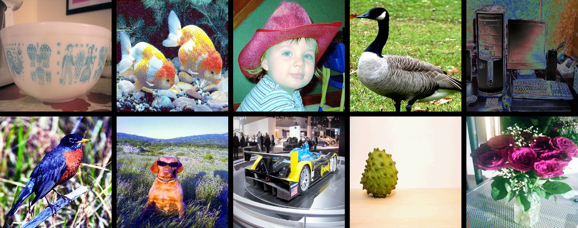
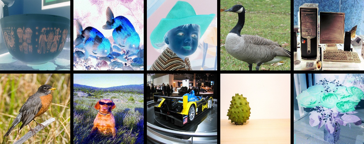
The images after AutoAugment are as follows.

3.1.3.2. RandAugment

Address: https://arxiv.org/pdf/1909.13719.pdf

Github repo: https://github.com/heartInsert/randaugment

The search method of AutoAugment is relatively violent. Searching for the optimal strategy for this data set directly on the data set requires a lot of computation. In RandAugment, the author found that on the one hand, for larger models and larger datasets, the gains generated by the augmentation method searched using AutoAugment are smaller. On the other hand, the searched strategy is limited to certain dataset, which has poor generalization performance and not sutable for other datasets.

In RandAugment, the author proposes a random augmentation method. Instead of using a specific probability to determine whether to use a certain sub-strategy, all sub-strategies are selected with the same probability. The experiments in the paper also show that this method performs well even for large models.

In PaddleClas, RandAugment is used as follows.

from ppcls.data.imaug import DecodeImage
from ppcls.data.imaug import ResizeImage
from ppcls.data.imaug import RandAugment
from ppcls.data.imaug import transform

size = 224

decode_op = DecodeImage()
resize_op = ResizeImage(size=(size, size))
randaugment_op = RandAugment()

ops = [decode_op, resize_op, randaugment_op]

imgs_dir = image_path
fnames = os.listdir(imgs_dir)
for f in fnames:
    data = open(os.path.join(imgs_dir, f)).read()
    img = transform(data, ops)

The images after RandAugment are as follows.

3.1.4. Image Cropping

Cropping means performing some transformations on the image after Transpose, setting pixels of the cropped area as certain constant. It mainly contains CutOut, RandErasing, HideAndSeek and GridMask.

Image cropping methods can be operated before or after normalization. The difference is that if we crop the image before normalization and fill the areas with 0, the cropped areas’ pixel values will not be 0 after normalization, which will cause grayscale distribution change of the data.

The above-mentioned cropping transformation ideas are the similar, all to solve the problem of poor generalization ability of the trained model on occlusion images, the difference lies in that their cropping details.

3.1.4.1. Cutout

Address: https://arxiv.org/abs/1708.04552

Github repo: https://github.com/uoguelph-mlrg/Cutout

Cutout is a kind of dropout, but occludes input image rather than feature map. It is more robust to noise than noise. Cutout has two advantages: (1) Using Cutout, we can simulate the situation when the subject is partially occluded. (2) It can promote the model to make full use of more content in the image for classification, and prevent the network from focusing only on the saliency area, thereby causing overfitting.

In PaddleClas, Cutout is used as follows.

from ppcls.data.imaug import DecodeImage
from ppcls.data.imaug import ResizeImage
from ppcls.data.imaug import Cutout
from ppcls.data.imaug import transform

size = 224

decode_op = DecodeImage()
resize_op = ResizeImage(size=(size, size))
cutout_op = Cutout(n_holes=1, length=112)

ops = [decode_op, resize_op, cutout_op]

imgs_dir = image_path
fnames = os.listdir(imgs_dir)
for f in fnames:
    data = open(os.path.join(imgs_dir, f)).read()
    img = transform(data, ops)

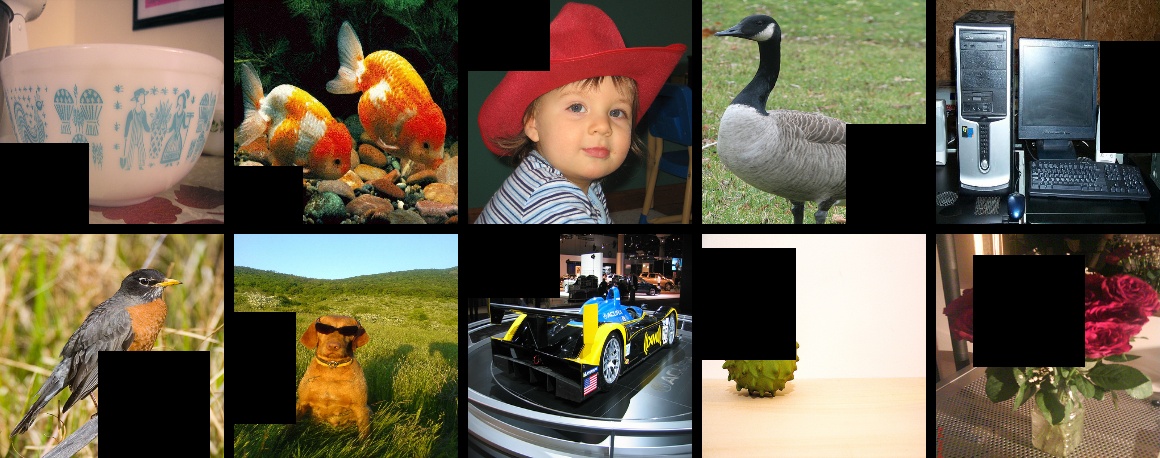
The images after Cutout are as follows.

3.1.4.2. RandomErasing

Address: https://arxiv.org/pdf/1708.04896.pdf

Github repo: https://github.com/zhunzhong07/Random-Erasing

RandomErasing is similar to the Cutout. It is also to solve the problem of poor generalization ability of the trained model on images with occlusion. The author also pointed out in the paper that the way of random cropping is complementary to random horizontal flipping. The author also verified the effectiveness of the method on pedestrian re-identification (REID). Unlike Cutout, in, RandomErasing is operateed on the image with a certain probability, size and aspect ratio of the generated mask are also randomly generated according to pre-defined hyperparameters.

In PaddleClas, RandomErasing is used as follows.

from ppcls.data.imaug import DecodeImage
from ppcls.data.imaug import ResizeImage
from ppcls.data.imaug import ToCHWImage
from ppcls.data.imaug import RandomErasing
from ppcls.data.imaug import transform

size = 224

decode_op = DecodeImage()
resize_op = ResizeImage(size=(size, size))
randomerasing_op = RandomErasing()

ops = [decode_op, resize_op, tochw_op, randomerasing_op]

imgs_dir = image_path
fnames = os.listdir(imgs_dir)
for f in fnames:
    data = open(os.path.join(imgs_dir, f)).read()
    img = transform(data, ops)
    img = img.transpose((1, 2, 0))

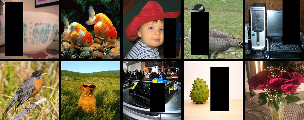
The images after RandomErasing are as follows.

3.1.4.3. HideAndSeek

Address: https://arxiv.org/pdf/1811.02545.pdf

Github repo: https://github.com/kkanshul/Hide-and-Seek

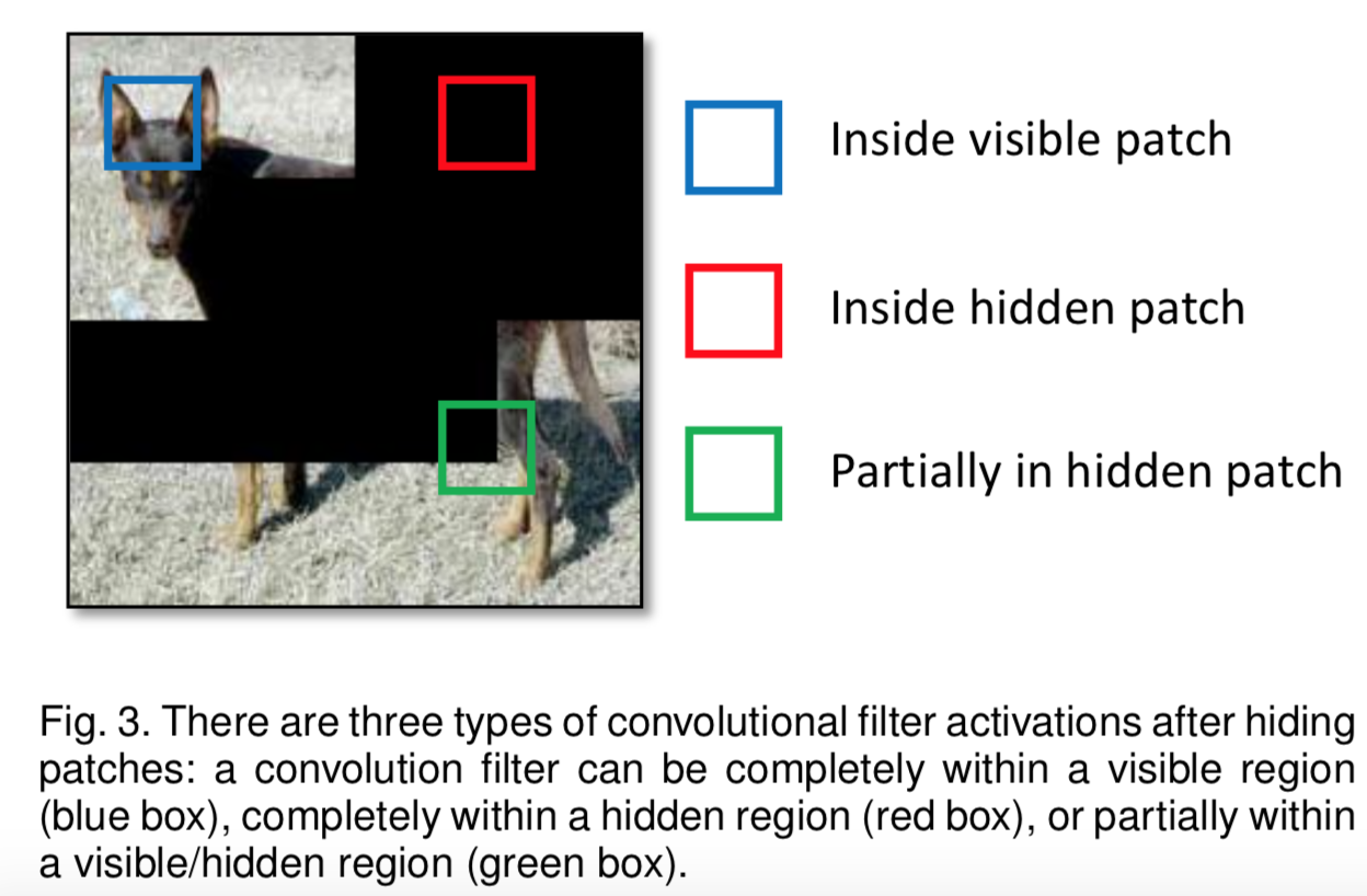
Images are divided into some patches for HideAndSeek and masks are generated with certain probability for each patch. The meaning of the masks in different areas is shown in the figure below.

In PaddleClas, HideAndSeek is used as follows.

from ppcls.data.imaug import DecodeImage
from ppcls.data.imaug import ResizeImage
from ppcls.data.imaug import ToCHWImage
from ppcls.data.imaug import HideAndSeek
from ppcls.data.imaug import transform

size = 224

decode_op = DecodeImage()
resize_op = ResizeImage(size=(size, size))
hide_and_seek_op = HideAndSeek()

ops = [decode_op, resize_op, tochw_op, hide_and_seek_op]

imgs_dir = image_path
fnames = os.listdir(imgs_dir)
for f in fnames:
    data = open(os.path.join(imgs_dir, f)).read()
    img = transform(data, ops)
    img = img.transpose((1, 2, 0))

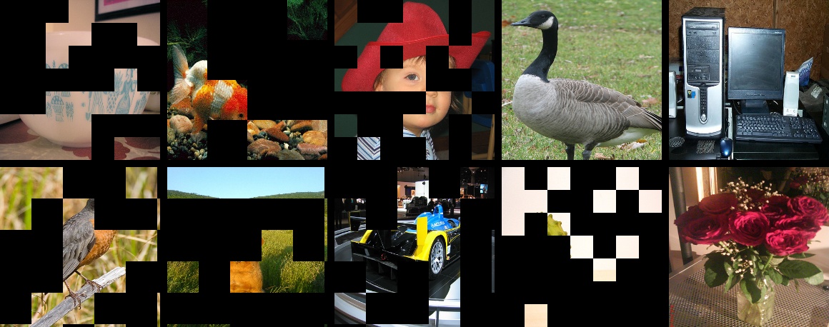
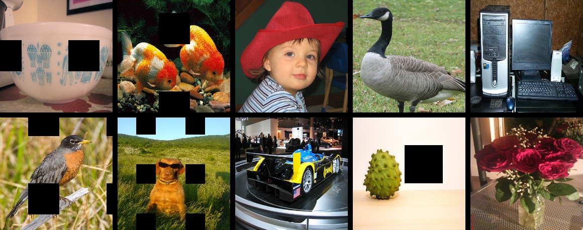
The images after HideAndSeek are as follows.

3.1.4.4. GridMask

Address：https://arxiv.org/abs/2001.04086

Github repo：https://github.com/akuxcw/GridMask

The author points out that the previous method based on image cropping has two problems, as shown in the following figure:

1. Excessive deletion of the area may cause most or all of the target subject to be deleted, or cause the context information loss, resulting in the images after enhancement becoming noisy data.
2. Reserving too much area has little effect on the object and context.

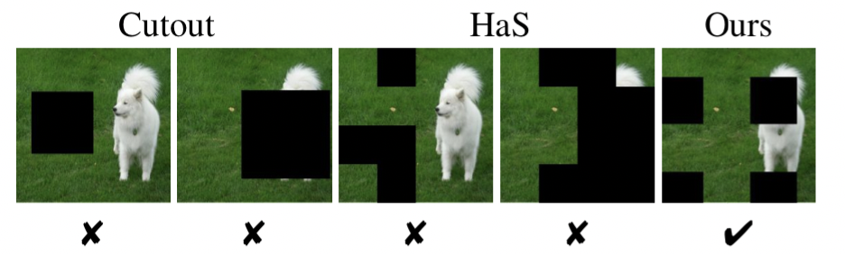
Therefore, it is the core problem to be solved how to if you avoid over-deletion or over-retention becomes the core problem to be solved.

GridMask is to generate a mask with the same resolution as the original image and multiply it with the original image. The mask grid and size are adjusted by the hyperparameters.

In the training process, there are two methods to use:

1. Set a probability p and use the GridMask to augment the image with probability p from the beginning of training.
2. Initially set the augmentation probability to 0, and the probability is increased with number of iterations from 0 to p.

It shows that the second method is better.

The usage of GridMask in PaddleClas is shown below.

from data.imaug import DecodeImage
from data.imaug import ResizeImage
from data.imaug import ToCHWImage
from data.imaug import GridMask
from data.imaug import transform

size = 224

decode_op = DecodeImage()
resize_op = ResizeImage(size=(size, size))
tochw_op = ToCHWImage()
gridmask_op = GridMask(d1=96, d2=224, rotate=1, ratio=0.6, mode=1, prob=0.8)

ops = [decode_op, resize_op, tochw_op, gridmask_op]

imgs_dir = image_path
fnames = os.listdir(imgs_dir)
for f in fnames:
    data = open(os.path.join(imgs_dir, f)).read()
    img = transform(data, ops)
    img = img.transpose((1, 2, 0))

The images after GridMask are as follows.

3.1.5. Image aliasing

Aliasing means performing some transformations on the image after Batch, which contains Mixup and Cutmix.

Data augmentation methods introduced before are based on single image while aliasing is carried on a certain batch to generate a new batch.

3.1.5.1. Mixup

Address: https://arxiv.org/pdf/1710.09412.pdf

Github repo: https://github.com/facebookresearch/mixup-cifar10

Mixup is the first solution for image aliasing, it is easy to realize and performs well not only on image classification but also on object detection. Mixup is usually carried out in a batch for simplification, so as Cutmix.

The usage of Mixup in PaddleClas is shown below.

from ppcls.data.imaug import DecodeImage
from ppcls.data.imaug import ResizeImage
from ppcls.data.imaug import ToCHWImage
from ppcls.data.imaug import transform
from ppcls.data.imaug import MixupOperator

size = 224

decode_op = DecodeImage()
resize_op = ResizeImage(size=(size, size))
tochw_op = ToCHWImage()
hide_and_seek_op = HideAndSeek()
mixup_op = MixupOperator()
cutmix_op = CutmixOperator()

ops = [decode_op, resize_op, tochw_op]

imgs_dir = image_path

batch = []
fnames = os.listdir(imgs_dir)
for idx, f in enumerate(fnames):
    data = open(os.path.join(imgs_dir, f)).read()
    img = transform(data, ops)
    batch.append( (img, idx) ) # fake label

new_batch = mixup_op(batch)

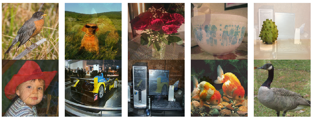
The images after Mixup are as follows.

3.1.5.2. Cutmix

Address: https://arxiv.org/pdf/1905.04899v2.pdf

Github repo: https://github.com/clovaai/CutMix-PyTorch

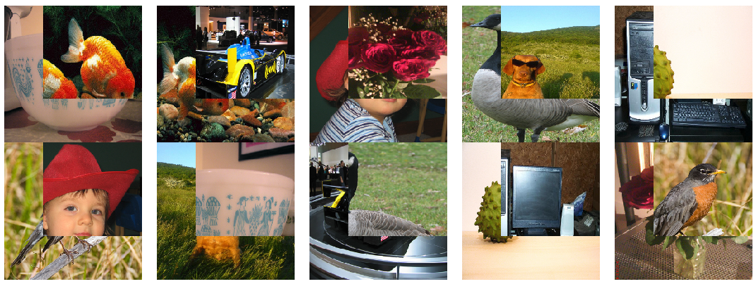
Unlike Mixup which directly adds two images, for Cutmix, an ROI is cut out from one image and Cutmix randomly cuts out an ROI from one image, and then covered onto the corresponding area in the another image. The usage of Cutmix in PaddleClas is shown below.

rom ppcls.data.imaug import DecodeImage
from ppcls.data.imaug import ResizeImage
from ppcls.data.imaug import ToCHWImage
from ppcls.data.imaug import transform
from ppcls.data.imaug import CutmixOperator

size = 224

decode_op = DecodeImage()
resize_op = ResizeImage(size=(size, size))
tochw_op = ToCHWImage()
hide_and_seek_op = HideAndSeek()
cutmix_op = CutmixOperator()

ops = [decode_op, resize_op, tochw_op]

imgs_dir = image_path

batch = []
fnames = os.listdir(imgs_dir)
for idx, f in enumerate(fnames):
    data = open(os.path.join(imgs_dir, f)).read()
    img = transform(data, ops)
    batch.append( (img, idx) ) # fake label

new_batch = cutmix_op(batch)

The images after Cutmix are as follows.

3.1.6. Experiments

Based on PaddleClas, Metrics of different augmentation methods on ImageNet1k dataset are as follows.

Model	Learning strategy	l2 decay	batch size	epoch	Augmentation method	Top1 Acc	Reference
ResNet50	0.1/cosine_decay	0.0001	256	300	Standard transform	0.7731	-
ResNet50	0.1/cosine_decay	0.0001	256	300	AutoAugment	0.7795	0.7763
ResNet50	0.1/cosine_decay	0.0001	256	300	mixup	0.7828	0.7790
ResNet50	0.1/cosine_decay	0.0001	256	300	cutmix	0.7839	0.7860
ResNet50	0.1/cosine_decay	0.0001	256	300	cutout	0.7801	-
ResNet50	0.1/cosine_decay	0.0001	256	300	gridmask	0.7785	0.7790
ResNet50	0.1/cosine_decay	0.0001	256	300	random-augment	0.7770	0.7760
ResNet50	0.1/cosine_decay	0.0001	256	300	random erasing	0.7791	-
ResNet50	0.1/cosine_decay	0.0001	256	300	hide and seek	0.7743	0.7720

note:

• In the experiment here, for better comparison, we fixed the l2 decay to 1e-4. To achieve higher accuracy, we recommend trying to use a smaller l2 decay. Combined with data augmentaton, we found that reducing l2 decay from 1e-4 to 7e-5 can bring at least 0.3~0.5% accuracy improvement.
• We have not yet combined different strategies or verified, whch is our future work.

3.1.6.1. Data augmentation practice

Experiments about data augmentation will be introduced in detail in this section. If you want to quickly experience these methods, please refer to Quick start PaddleClas in 30 miniutes.

3.1.6.2. Configurations

Since hyperparameters differ from different augmentation methods. For better understanding, we list 8 augmentation configuration files in configs/DataAugment based on ResNet50. Users can train the model with tools/run.sh. The following are 3 of them.

3.1.6.2.1. RandAugment

Configuration of RandAugment is shown as follows. Num_layers(default as 2) and magnitude(default as 5) are two hyperparameters.

    transforms:
        - DecodeImage:
            to_rgb: True
            to_np: False
            channel_first: False
        - RandCropImage:
            size: 224
        - RandFlipImage:
            flip_code: 1
        - RandAugment:
            num_layers: 2
            magnitude: 5
        - NormalizeImage:
            scale: 1./255.
            mean: [0.485, 0.456, 0.406]
            std: [0.229, 0.224, 0.225]
            order: ''
        - ToCHWImage:

3.1.6.2.2. Cutout

Configuration of Cutout is shown as follows. n_holes(default as 1) and n_holes(default as 112) are two hyperparameters.

    transforms:
        - DecodeImage:
            to_rgb: True
            to_np: False
            channel_first: False
        - RandCropImage:
            size: 224
        - RandFlipImage:
            flip_code: 1
        - NormalizeImage:
            scale: 1./255.
            mean: [0.485, 0.456, 0.406]
            std: [0.229, 0.224, 0.225]
            order: ''
        - Cutout:
            n_holes: 1
            length: 112
        - ToCHWImage:

3.1.6.2.3. Mixup

Configuration of Mixup is shown as follows. alpha(default as 0.2) is hyperparameter which users need to care about. What’s more, use_mix need to be set as True in the root of the configuration.

    transforms:
        - DecodeImage:
            to_rgb: True
            to_np: False
            channel_first: False
        - RandCropImage:
            size: 224
        - RandFlipImage:
            flip_code: 1
        - NormalizeImage:
            scale: 1./255.
            mean: [0.485, 0.456, 0.406]
            std: [0.229, 0.224, 0.225]
            order: ''
        - ToCHWImage:
    mix:
        - MixupOperator:
            alpha: 0.2

3.1.6.3. 启动命令

Users can use the following command to start the training process, which can also be referred to tools/run.sh.

export PYTHONPATH=path_to_PaddleClas:$PYTHONPATH

python -m paddle.distributed.launch \
    --selected_gpus="0,1,2,3" \
    tools/train.py \
        -c ./configs/DataAugment/ResNet50_Cutout.yaml

3.1.6.4. Note

• When using augmentation methods based on image aliasing, users need to set use_mix in the configuration file as True. In addition, because the label needs to be aliased when the image is aliased, the accuracy of the training data cannot be calculated. The training accuracy rate was not printed during the training process.
• The training data is more difficult with data augmentation, so the training loss may be larger, the training set accuracy is relatively low, but it has better generalization ability, so the validation set accuracy is relatively higher.
• After the use of data augmentation, the model may tend to be underfitting. It is recommended to reduce l2_decay for better performance on validation set.
• hyperparameters exist in almost all agmenatation methods. Here we provide hyperparameters for ImageNet1k dataset. User may need to finetune the hyperparameters on specified dataset. More training tricks can be referred to Tricks.

If this document is helpful to you, welcome to star our project: https://github.com/PaddlePaddle/PaddleClas

3.1.7. Reference

[1] Cubuk E D, Zoph B, Mane D, et al. Autoaugment: Learning augmentation strategies from data[C]//Proceedings of the IEEE conference on computer vision and pattern recognition. 2019: 113-123.

[2] Cubuk E D, Zoph B, Shlens J, et al. Randaugment: Practical automated data augmentation with a reduced search space[J]. arXiv preprint arXiv:1909.13719, 2019.

[3] DeVries T, Taylor G W. Improved regularization of convolutional neural networks with cutout[J]. arXiv preprint arXiv:1708.04552, 2017.

[4] Zhong Z, Zheng L, Kang G, et al. Random erasing data augmentation[J]. arXiv preprint arXiv:1708.04896, 2017.

[5] Singh K K, Lee Y J. Hide-and-seek: Forcing a network to be meticulous for weakly-supervised object and action localization[C]//2017 IEEE international conference on computer vision (ICCV). IEEE, 2017: 3544-3553.

[6] Chen P. GridMask Data Augmentation[J]. arXiv preprint arXiv:2001.04086, 2020.

[7] Zhang H, Cisse M, Dauphin Y N, et al. mixup: Beyond empirical risk minimization[J]. arXiv preprint arXiv:1710.09412, 2017.

[8] Yun S, Han D, Oh S J, et al. Cutmix: Regularization strategy to train strong classifiers with localizable features[C]//Proceedings of the IEEE International Conference on Computer Vision. 2019: 6023-6032.